PCA, EigenFace and All That
PCA(Principal Component Analysis) is one of the most commonly used unsupervised learning algorithm to compress, extract features for data and even for dimensionality reduction purposes. It has quite a lof of applications as follows:
Applications
- Useful for compression and classfication of data.
- Aim is to reduce the number of variables, but at the same time, preserve most of information (variation), which may not necessarily hold true in general.
- New variables called principal components(PC) are uncorrelated, are ordered by fraction of total information each retains.
- PC’s are a series of linear least squares fits to a sample, each orthogonal to all previous.
- Identify how different variables work together to create the dynamics of the system.
- Reduce the dimensionality of the data.
- Decrease the redundancy of the data.
- Filter some of the noise in the data.
- Compress the data.
- Prepare the data for further analysis using other techniques.
What does it do in the first place?
Functions of PCA
- Is to reduce dimensionality by extracting the smallest number components that account for most of the variation in the original data. By doing so, we’d get get rid of the redundancy and preserve the variance in a smaller number of coefficients.
- PCA finds lines(2-d), planes(3-d) in a higher dimensional spaces that approximate the data in least squares( norm).
Why do we choose PCA over other transformations which turn the original variables into a representation which depend on orthogonal bases, say Fourier Transform?
- Using a set of fixed set of components will give a good reconstruction of the same data(at least in least square sense, norm). However, Fourier transform does not guarantee such a premise.
- If the data has a lot of correlation among its variables(redundancy), then PCA could exploit this redundancy by uncorrelating the variables whereas Fourier transform cannot exploit this redundancy(at least explicitly).
- When PCA is used for dimensionality reduction, it is quite good at preserving the distance between the observations in the projection space.
What about the disadvantages?
- The components are not independent but uncorrelated. It would be even better if we have a representation which are independent to each other. It is called unsurprisingly Independent Component Analysis.
- PCA seeks for linear combinations of the original variables. The nonlinear combination may even yield better representation. PCA has an extension for doing this type of analysis, Nonlinear PCA.
- Instead of norm, it may be advantageous to use norm. Especially, if the signal that we want to represent is sparse or has a sparse representation in some other space. PCA is extended for this specific problem as well, which is called Sparse PCA.
Assumptions that PCA does:
- Assumption 1: In general, high correlation between variables could be a sign of high redundancy.
- Assumption 2: The most important dynamics are the ones with the largest variance.
Eigenvalues and Eigenvectors
- Eigenvalues measure the amount of variation(information) explaiend by each principal components and will be largest for the first PC and smaller for the subsequent PCs.
- An eigenvalue greater than 1 indicates that principal component accounts for more variance than accounted by one of the original variables in standardized data. This could be used to threshold to determine the number of eigenvectors.
- Eigenvectors provide the weights to compute the uncorrelated principal components, which are the linear combination of the original variables.
What does PCA do (in a nutshell)?
- PCA transforms the observations into uncorrelated components, which are nothing but linear combination of observations.
Caveats
- PCA is sensitive to scaling.
By modifying the variance of the variables(scaling), it is possible to attribute different importance to them. By doing so, the prior information or the belief on the importance of the attributes can be preserved even in the PCA stage.
Definition of Principal Components
Given a sample observations on a vector variables:
define the principal component of the sample by a linear transformation which is given as following:
where is which is chosen to maximize the variance of and subject to and to
How to derive the coefficients ?
The variance is:
where is the covariance matrix for .
To find which maximizes subject to , let us introduce a lagrange multiplier . Then, the maximization equation becomes If we take the derivative with respect to , then the equation becomes Therefore, is an eigenvector of which has the corresponding value of .
In short, we are interested in representing the most of the variation in the data by transforming the original variables into principal components. These components are orthogonal and ordered by magnitude so that the first few of them could explain most of the variation in the original observation.
EigenFace
PCA has a very good application which is in the computer vision domain, called EigenFace, short version. Eigenface is a name for eigenvectors which are the components of the face itself. It has been used for face recognition where the most variations considered as important. It was quite successful as well for some 20 years ago although it was replaced then by other methods. In this implementation, I used a particular subset of Yale Face Database.
The images that I used are given below: 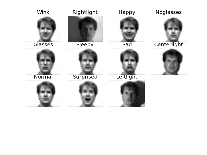
If we average the face used for PCA, we get the following face: 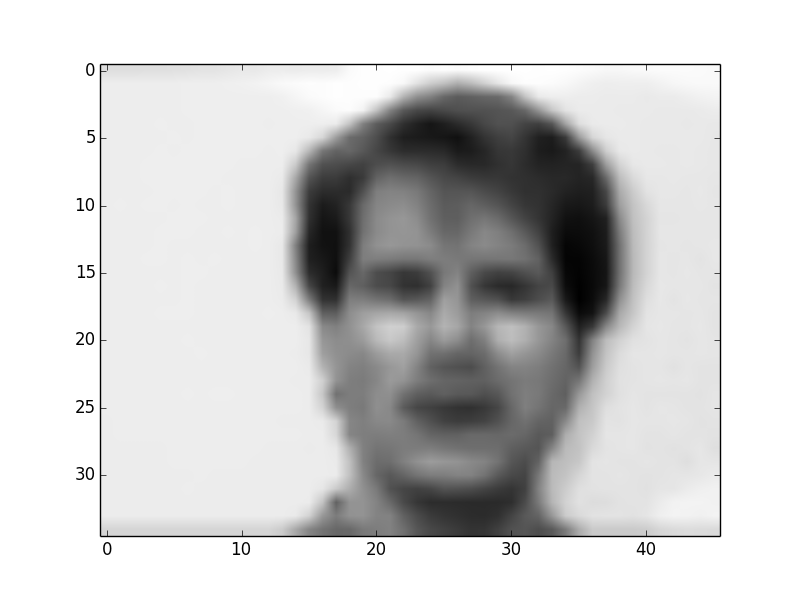
The eigenfaces that we generated out of 11 faces are given below. 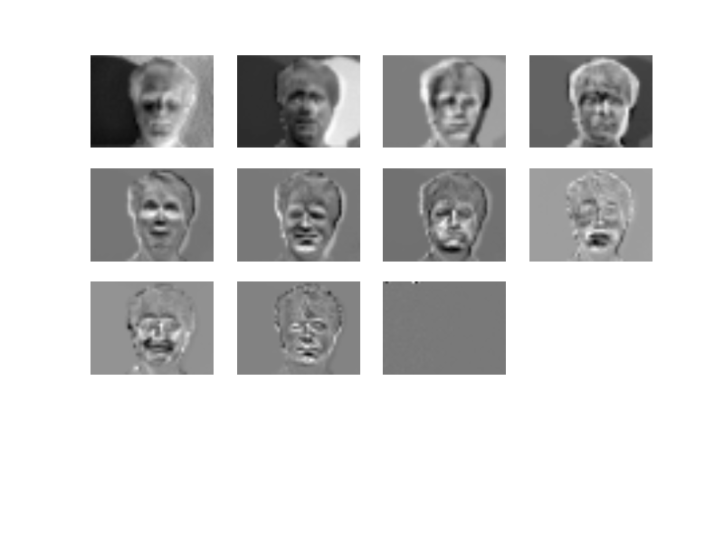
The eigenface which has the most variation(almost half of it) is given below(note the illumination variation) 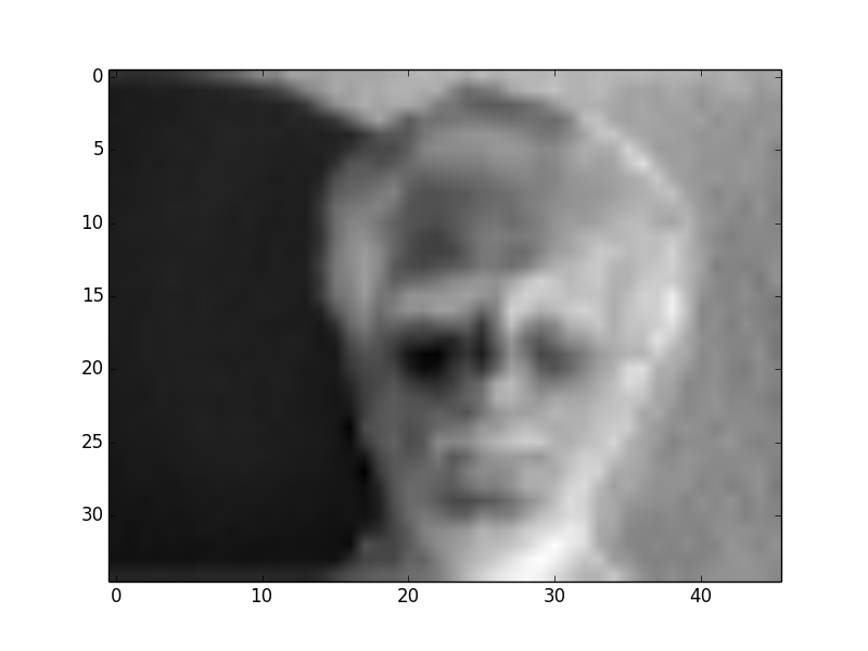
Cumulative sum of first 10 eigenvalues is given below. 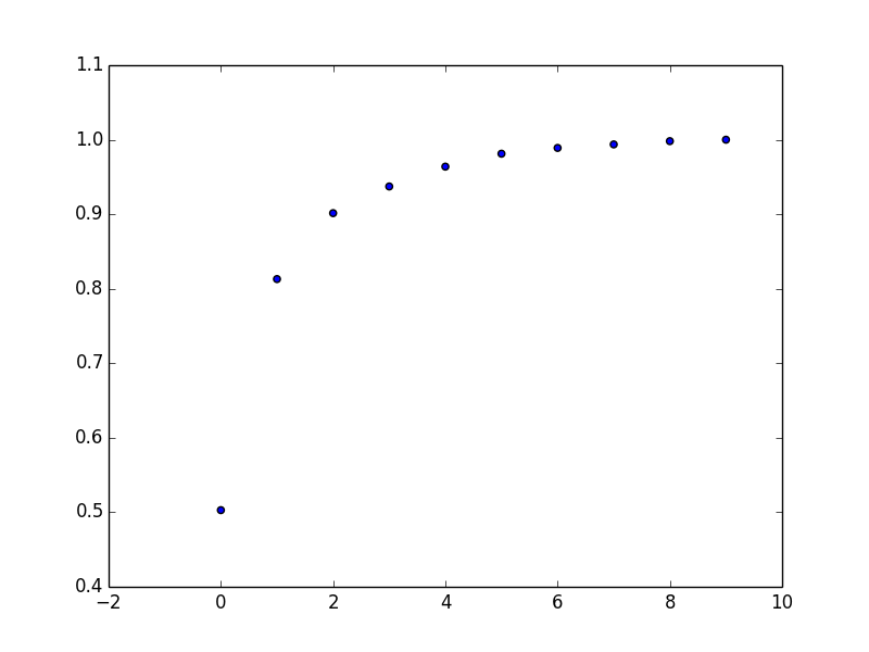
As it could be seen from here(the last line), the top 4 eigenfaces can explain 95% variance of the faces.
The program that I used to generate the images in here and see the Notebook for the flow of overall program.